Optimisation of material composition in functionally graded plates for thermal stress relaxation using statistical design support system
-
Ryoichi Chiba
 and
Yoshihiro Sugano
and
Yoshihiro Sugano

Abstract
This study addresses the optimisation of material composition in a functionally graded plate for thermal stress relaxation, subjected to through-thickness thermal gradients, with the aim of minimising a stress utilisation ratio. We simplify the problem by approximating the functionally graded plate as a multi-layered plate. Material compositions in individual layers are optimised using a statistical design support system (SDSS), incorporating design of experiments and mathematical programming techniques. The volume fractions of ceramic constituent in the respective layers are considered as design variables, and an analytical solution for transient thermal stresses is utilised to evaluate the objective function. The optimisation results obtained using the SDSS are compared with those from a genetic algorithm (GA) to validate the applicability of the proposed method. Our findings indicate that the SDSS replicates the ceramic volume fraction distribution optimised by the GA, while significantly reducing optimisation time.
1 Introduction
Functionally graded materials (FGMs) are advanced materials designed to fulfil specific functions such as thermal stress relaxation, biological compatibility, and refractive index control. These functions are achieved through either a spatially continuous or finely stepwise variation in the material composition and/or microstructure. FGM is often termed a “designable material.” To fully exploit the potential of FGMs, they should be fabricated with an optimal material composition distribution, tailored to the specific environment in which they will be used.
In a survey of optimal material composition design methods for FGMs, several techniques have been reported with a focus on thermal stress relaxation. Regarding the setting of design variables, Ootao et al. [1] constrained the material composition distribution to follow a power-law function of a spatial coordinate and optimised the exponent using neural networks. Similarly, Na and Kim [2] conducted an optimisation of this nature using the quasi-Newton’s method. However, the resulting composition distributions are not exactly optimal because of the constraints. To derive an optimal composition distribution without such constraints, Ootao et al. [3] and Sugano et al. [4] modelled an FGM as a multi-layered body in which each layer was homogeneous or linearly non-homogeneous, respectively. They then used a genetic algorithm (GA) to find the optimal material composition for each layer. Surendranath et al. [5] and Moleiro et al. [6] enhanced the efficiency of optimisation computations by treating the thicknesses of pure material layers and a power-law function exponent for the graded layer, rather than the individual layer compositions, as design variables.
When it comes to optimisation algorithms, gradient-based approaches including sequential quadratic programming [7,8,9] and metaheuristic approaches such as differential evolution [10], GA [3,11,12,13,14], particle swarm optimisation [15,16,17], and simulated annealing [18] have mainly been employed. However, metaheuristic approaches can be time-consuming, often requiring numerous iterations and objective function evaluations to converge to a solution. The computational cost can be particularly high if the objective function itself is complex and computationally intensive, such as when transient analysis is necessary.
To alleviate the computational load associated with optimisation, this study employs a statistical design support system (SDSS), developed by Kashiwamura et al. [19], to solve the material composition optimisation problem for FGMs. The SDSS is a practical and efficient tool for large-scale, multilevel, and multidisciplinary optimisation tasks. It has been successfully applied to reduce the manufacturing costs [19] and weight [20] of vehicle seat frames, while maintaining requisite safety standards. It has also been used for the shape design of plastic bottles [21] and the structural optimisation of electrostatically actuated micromirrors [22].
In this study, a thermally loaded FGM plate is approximated as a multi-layered structure, with each layer’s material composition treated as design variables. Using the SDSS, we aim to find a composition distribution that minimises the maximum stress utilisation ratio – the ratio of thermal stress to strength in the FGM plate. The validity of this approach is further evaluated in terms of optimisation time and the accuracy of the optimal solution, through a comparison with results obtained using a GA.
2 Analytical approach for evaluating thermal stress
Our analysis focuses on a fully dense FGM plate, which is characterised by widths significantly larger than its thickness. This plate is completely free of surface traction, and its major surfaces are subjected to uniform thermal loading. Such a configuration ensures a predominantly one-dimensional heat flow. Additionally, we address transient thermal stress, which is crucial for evaluating the FGM plate’s performance under operational conditions.
2.1 Temperature field
As an analytical model, let us consider an infinite FGM plate in which the thermal conductivity λ, density ρ, specific heat c, Young’s modulus E, coefficient of linear thermal expansion α, and Poisson’s ratio ν vary arbitrarily along the thickness direction, or the z-axis. Assuming temperature-independent material properties and no heat generation within the plate, the one-dimensional heat conduction equation along the z-axis is expressed as follows:
Eq. (1) is a differential equation with variable coefficients; therefore, it is very difficult to obtain an exact solution for arbitrary non-homogeneity in λ, ρ and c. To solve Eq. (1), we divide the plate into n layers along the z-axis, approximating the continuous variation in material properties with distinct constants within each layer. This approximation facilitates the analysis of the transient heat conduction.
Figure 1 illustrates the analytical model. An infinite plate of thickness h, exhibiting non-homogeneity along the thickness direction (z-axis), is in contact with surrounding media at temperatures θ 1(t) and θ 2(t) at z = 0 and z = h, respectively. The heat transfer coefficients for the plate’s surfaces are h 1 and h 2. The plate is segmented into n layers, and the positions of the imaginary interfaces within the plate are denoted as a i (i = 1, 2,…, n − 1). We assume an initial plate temperature of zero.

Analytical model representing an infinite FGM plate, approximated as a multi-layered body.
In this case, the transient heat conduction problem for the FGM plate can be formulated as follows:
The analytical solution of the heat conduction problem is now derived by applying Vodicka’s method [23,24]. This method provides an eigenfunction-based series solution that uses quasi-orthogonality [25] of the eigenfunctions. Following the method, the form of the solution to Eqs (2)–(6) is assumed to be
where
Eigenfunction X im (z) is the solution to the eigenvalue problem and is given as follows:
where κ i is the thermal diffusivity defined as κ i = λ i /(ρ i c i ). The conditions necessary for determining the unknown coefficients A im , B im , C ij , and D ij can be obtained by substituting Eq. (7) into Eqs (4)–(6). Eigenvalues γ m (m = 1, 2,…) are obtained from the condition under which A im and B im are both non-zero and are therefore the positive roots of the following transcendental equation:
where
The eigenfunction X
im
(z) has the following quasi-orthogonal relationship with the discontinuous-weighting function
Applying the orthogonal-expansion technique based on Eq. (14), we obtain the time function ϕ m (t) as follows:
where
2.2 Thermal stress field
Sugano [26] derived an expression for in-plane thermal stresses in plates that are non-homogeneous across their thickness. The expression is applicable where the temperature varies only along the thickness direction, i.e. T = T(z), and the boundary surfaces are free of tractions. This expression is given as follows:
where
Eq. (17) was derived through a two-step process: (i) first, by determining the form of stress components to satisfy the compatibility equations expressed in terms of stress components; and (ii) second, by identifying two unknown constants so that the resultant force and moment (per unit length) produced by σ xx and σ yy are zero over the edges of the plate. According to Saint-Venant’s principle, Eq. (17) provides an accurate approximation for traction-free edges at distances from these edges greater than approximately one plate thickness [26].
In this study, we utilise this expression to analyse the thermal stress field. Eq. (17) can be directly applied to evaluate thermal stresses in multi-layered plates, as the plates can be viewed as non-homogeneous structures, with their material properties varying in a stepwise manner along the thickness direction.
3 SDSS
The SDSS, noted for its efficiency, versatility, and practical utility, is an optimisation tool that employs a type of response surface method. A detailed explanation of the SDSS can be found in the study by Kashiwamura et al. [19], but for convenience, we provide a brief summary here. The system comprises two main parts: the effectivity analysis and the optimisation calculation.
3.1 Effectivity analysis
The effect of design variables on a characteristic value (objective function) is quantitatively obtained through a limited number of analyses by combining the design of experiments and structural analysis, which corresponds to the thermal stress analysis in this study. The process of effectivity analysis includes the following steps:
An upper limit and a lower limit are set for each design variable, and discrete points are generated within this range at regular intervals. The number of discrete points, the span between the upper and lower limits and the interval between discrete points are referred to as the “number of levels,” the “range of level values,” and the “interval between levels,” respectively.
The most appropriate orthogonal array is selected based on the number of design variables, the interaction setting between the design variables and the number of levels.
In the orthogonal array, the design variables are assigned to the columns, while the input data for the structural analysis are assigned to the rows according to the design of experiments.
Structural analysis is performed using the input data assigned to the orthogonal array, and the characteristic value data are obtained for the analysis of variance (ANOVA).
The ANOVA is conducted, and an estimation expression for the characteristic value obtained from the structural analysis is prepared. The ANOVA uses an evaluation method that decomposes the effect of design variables on the characteristic value into orthogonal components. The estimation expression for each design variable is provided by an orthogonal polynomial, represented by Chebyshev’s orthogonal function as follows:
where A represents a design variable,
3.2 Optimisation calculation
In the present method, optimisation is performed using the estimation expression derived from the effectivity analysis, enabling the use of a relatively straightforward algorithm. Specifically, the aforementioned estimation expression serves as the objective function for optimisation, and the optimisation calculation is carried out using mathematical programming under suitable constraint conditions.
The accuracy of the optimal solution obtained depends heavily on the accuracy of the estimation expression in the SDSS. As the estimation expression is a regression equation within the range of level values of the design variables, constraining this range can enhance the accuracy of the estimation expression. To lessen the influence of the range of level values on the estimation expression’s accuracy, this study employs a multi-stage analysis, which is briefly explained below.
The multi-stage analysis proceeds as follows: Initially, a broad range of level values is set, and the creation of the estimation expression and the optimisation calculation are conducted. Subsequently, based on the optimisation results, the range of level values for each design variable is revised, and the effectivity analysis and the optimisation calculation are repeated. This iterative process serves to improve the accuracy of the estimation expression.
4 Numerical calculation
In this study, we approximate a metal/ceramic FGM plate as a multi-layered plate composed of ten layers. Using the SDSS, the optimal material composition distribution for thermal stress relaxation is determined. A five-stage analysis is implemented to enhance the accuracy of the estimation expression. Additionally, the optimisation process is conducted using the GA, providing a comparative assessment with the results obtained from the SDSS.
4.1 Design of experiments
The volume fractions of ceramic in layers 2–9, denoted as V 2, V 3,…, V 9, are considered as design variables for the optimisation, while the first and tenth layers are assumed to be pure metal and pure ceramic, respectively. Consequently, the optimisation problem involves eight design variables. Regarding the number of levels, a four-level system is used, enabling the characteristic to be expressed as a third-degree equation. The interaction between the design variables is assumed to be negligible, leading to the selection of the orthogonal array L64(421) as the most appropriate one.
In the first stage, we set the lower and upper limits for each design variable, denoted as
where
4.2 Thermal stress analysis
To take the generality of the analysis into account, we introduce the following dimensionless coordinate and Fourier number:
In terms of heat load conditions on the FGM plate, we assume the surface temperatures at ζ = 0 and ζ = 1 for τ > 0 to be zero and a constant temperature T
0, respectively (For convenience in our computations, we set T
0 = 400.) The FGM used for thermal stress relaxation in the numerical calculations is composed of aluminium alloy (A7075) and alumina (Al2O3). Table 1 presents the material properties of aluminium alloy and alumina [28], where
Material properties of A7075 and Al2O3 [28]
| Material properties | A7075 | Al2O3 |
|---|---|---|
| λ (W·m–1·K–1) | 154 | 36 |
| ρ (kg·m–3) | 2,800 | 3,990 |
| c (J·kg–1·K–1) | 963 | 758 |
| α (× 10–6 K–1) | 23.0 | 8.0 |
| E (GPa) | 73 | 343 |
| σ Bt (MPa) | 485.0 | 259.7 |
| σ Bc (MPa) | 1940.0 | 2930.2 |
| ν (−) | 0.33 | 0.22 |
With respect to the FGM’s effective material properties, the density, specific heat, and Poisson’s ratio are estimated using the linear rule of mixtures. The thermal conductivity, coefficient of linear thermal expansion, and Young’s modulus, on the other hand, are calculated using a combination of Mori–Tanaka’s theory [29] – which provides accurate estimates of homogenised material properties when spherical inclusions are dispersed in a matrix – and fuzzy inference [24]. The tensile and compressive strengths are simply estimated by the linear rule of mixtures owing to the absence of a reliable estimation method for the strength of multi-phase materials, based on the microstructure.
4.3 ANOVA and optimisation
The key characteristic in our ANOVA and estimation expression is the maximum value of the stress utilisation ratio f [28], given by the following equation:
The ratio f represents the ratio between the absolute value of stress produced at any given position within the FGM plate and the tensile or compressive strength at the same point. In our numerical calculations, we estimate the maximum value of f (f max) by computing f at 11 equally spaced discrete points within each layer and 6 discrete Fourier numbers (τ = 0.001 × 5 i ; i = 0, 1,…, 5).
Using the estimation expression for f max derived from the ANOVA, we determine the material composition distribution that minimises f max. The constraints applied include side constraints and the requirement for the ceramic volume fraction to increase with the value of ζ. Consequently, the optimisation problem is formulated as follows:
where
4.4 GA
The volume fractions of the ceramic in the second to the ninth layers are coded as genes composed of 6-bit binary numbers. Table 2 presents the specifications of the GA used in the optimisation. The fitness function F, which acts as the criterion for determining individuals to survive in the next generation, is defined as follows:
Specifications of the GA utilised for the material composition optimisation
| GA parameter | Values or methods adopted |
|---|---|
| Length of bit strings | 48 |
| Population size | 80 |
| Selection | Roulette strategy and Elitism |
| Crossover/probability | Uniform crossover/0.75 |
| Mutation/probability | One-point mutation/0.01 |
| Scaling | Power scaling |
When the power-scaling coefficient hits 10 and no change is observed in the best individual for another 10 generations, we consider the calculation to be complete. The parameter combination in Table 2 produces the optimal solution in our numerical experiments among several parameter combinations tested.
5 Numerical results and discussion
The optimal volume fraction distribution obtained through the GA is presented first, as seen in Figure 2(a). To achieve this optimisation, a total of 122 generations were required in the GA. The volume fraction distribution shown in this figure takes on an S-shape, a complex pattern not easily expressed by a simple function, such as a power-law type or an exponential function. This volume fraction distribution is treated as a reference solution for a potentially optimal solution.

(a) Through-thickness distribution of the volume fraction of alumina, optimised by the GA, (b) corresponding transient thermal stress distributions across the thickness, (c) transient stress utilisation ratio distributions across the thickness, and (d) time evolution of the maximum stress utilisation ratio within the plate and the position of its occurrence.
For the FGM plate that exhibits the volume fraction distribution depicted in Figure 2(a), the value of f max is 0.763. The corresponding transient distributions of the thermal stress and stress utilisation ratio are presented in Figure 2(b) and (c), respectively. Meanwhile, Figure 2(d) illustrates the maximum stress utilisation ratio within the plate at each elapsed time, along with the position of its occurrence, which aligns with the depiction in Figure 2(c). Plots with empty circles mark the sampling points at discrete Fourier numbers used for the f max search.
Second, in the multi-stage analysis with B = 0.3 in Eq. (20), the results obtained from the optimisation of each stage, from the first to the third, are presented in Figure 3. The range of level values for each design variable in the next stage is also shown in Figure 3. When compared with Figure 2(a), it can be observed that the range of level values for the design variables in the third stage is very narrow as demonstrated in Figure 3(b); hence, the reference optimal values of V 3 and V 4 (i.e. 0.123 and 0.138) fall outside this range of level values. As a result, the reference optimal solution may not be achievable. This implies that in the multi-stage analysis, an excessively large restriction on the range of level values in the early stages or a very small value of B in Eq. (20) yields solutions that significantly deviate from the reference optimal solution. This occurs when the optimal values of the design variables lie outside the designated search area.

Stage-by-stage distribution of volume fraction optimised by the SDSS with B = 0.3: (a) first stage, (b) second stage, and (c) third stage.
Third, another multi-stage analysis is conducted with B = 0.5 in Eq. (20). Figure 4 presents the results obtained from the optimisation calculation for each stage. In addition, a recalculation of f
max with the analytical solution is carried out for each volume fraction distribution depicted in Figure 4. The f
max obtained from the estimation expression and that recalculated with the analytical solution are defined as
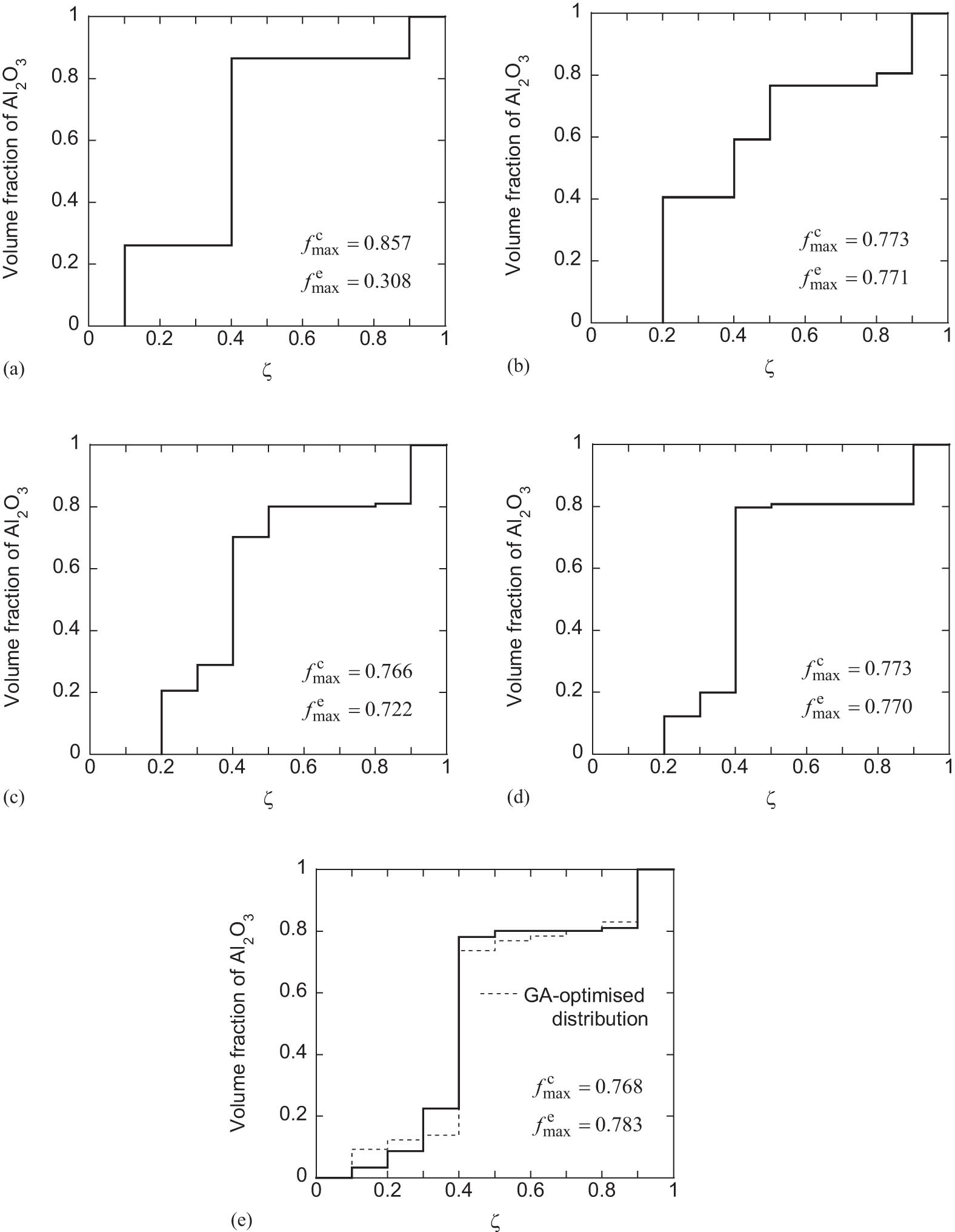
Stage-by-stage distribution of volume fraction optimised by the SDSS with B = 0.5, along with corresponding values of
Figure 4 illustrates a rapidly increasing volume fraction in the fifth layer, a feature that appears in the early stages of the multi-stage analysis. With an increase in the stage number, the change step of the volume fraction becomes finer towards the cooling side. Ultimately, this converges to an S-shaped volume fraction distribution. A good agreement is observed between the distribution tendencies in Figures 2(a) and 4(e). The difference in f max between these figures is relatively minor, standing at only 0.005. As depicted in Figure 5, the distributions of the stress utilisation ratio at transient states show minor differences between the FGM plate with material composition optimised by the SDSS and the GA-optimised counterpart. The value of max ζ ∊ [0,1] f(ζ) exhibits the most significant difference at the steady state.
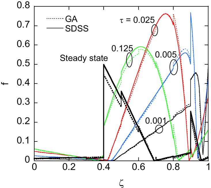
Comparison of the transient stress utilisation ratio distributions between the FGMs optimised by the SDSS (B = 0.5) and GA; solid curves represent the results for the SDSS, while dotted curves represent the GA results.
When comparing Figures 4(a) and 2(a), a large difference in the characteristic value f
max becomes apparent. The
The estimation expression for the characteristic value, f max, based on the ANOVA in the fifth stage with B = 0.5, is given as follows:
where the parameters are detailed in Table 3. This expression has been utilised in the optimisation calculation, resulting in the volume fraction distribution shown by the solid line in Figure 4(e). The estimation expression is a simple multivariate polynomial with design variables – specifically, volume fractions from the second to the ninth layers – serving as variables. Eq. (25) is a third-degree equation for each variable, as four levels of design variables are used in the design of experiments.
Parameters of the estimation expression Eq. (25)
| i | pi | qi | ri |
|---|---|---|---|
| 2 | 1.009608 | –43.01955 | 559.9773 |
| 3 | –0.0430842 | 0.3880247 | –1.041754 |
| 4 | 0.328694 | –1.664528 | 2.773205 |
| 5 | –4.487435 | 5.631629 | –2.354949 |
| 6 | 1.025061 | –1.302143 | 0.5261735 |
| 7 | 107.4804 | –130.1197 | 52.40004 |
| 8 | 123.6146 | –166.291 | 74.26361 |
| 9 | 130.7737 | –169.431 | 73.00222 |
To assess the accuracy of the estimation expression for f max at each stage, the estimation error, ε, is introduced as a performance index for the estimation accuracy:
Additionally, the approximate average estimation error for the estimation expression at each stage, ε av, is presented in Figure 6 (refer to the appendix for the definition of ε av). Reviewing Figure 4, it can be noted that the estimation error ε does not necessarily decrease as the stage number increases. However, ε av does decrease with an increase in the stage number, amounting to only about 1% in the fifth stage. Thus, despite the simplicity of Eq. (25) being a third-degree estimation expression, it is capable of estimating the characteristic value f max with considerable accuracy.

Histogram showing the average estimation error for f max at each stage with B = 0.5.
Concerning the calculation time required in the optimisation process, the GA optimisation necessitates 122 generations, equivalent to 9,760 executions of the transient thermal stress analysis routine. In contrast, the five-stage SDSS only requires the routine to be performed 320 times. Consequently, it becomes feasible to obtain a volume fraction distribution that closely mirrors the reference optimal solution in a drastically reduced time frame – approximately 3% of the time required by GA optimisation. This advantage becomes particularly significant in the material design of more complex shell-type structures made of FGMs [30,31] or multilayers [32].
6 Conclusion
This study has applied the SDSS, as proposed by Kashiwamura et al. [19], to optimise the material composition of FGMs for thermal stress relaxation. Our approach focused on a ten-layered FGM plate composed of aluminium alloy and alumina, evaluating the method’s effectiveness in terms of solution accuracy and computational efficiency.
We found that a single-stage SDSS is inadequate for approximating the potentially optimal solution provided by the GA. This necessitates the use of a multi-stage SDSS, where a strategic adjustment of the range of level values is crucial. Particularly, we observed that for optimal material composition design of FGMs, modifying the range of level values in line with Eq. (20) is essential. A B parameter value below 0.5 proved ineffective for aligning with the GA’s optimal solution. Furthermore, our method, with a gradually decreasing range of level values, successfully approximated the volume fraction distribution close to the potentially optimal one, while markedly reducing computational time compared to the GA optimisation.
The method’s reliance on orthogonal arrays limits the number of design variables, and the accuracy of the estimation expression is dependent on the number of levels and the range of level values. However, our approach substantially lowers the computational burden, facilitating rapid optimisation. It also offers valuable insights into the impact of design variables on characteristic values, which is advantageous for FGM design.
While the optimal solution obtained is approximate, this method paves the way for rapid and efficient optimisation, and it holds promise for extension to multi-objective optimisations, as indicated by Yu et al. [33], crucial for designing more multi-functional FGMs.
-
Funding information: The authors state no funding involved.
-
Author contributions: All authors have accepted responsibility for the entire content of this manuscript and approved its submission.
-
Conflict of interest: The authors state no conflict of interest.
-
Data availability statement: The data that support the findings of this study are available from the corresponding author, R.C., upon reasonable request.
Appendix
Considering that the design variables V 2, V 3,…, V 9 are continuous variables, the average estimation error for the estimation expression with respect to f max is defined as follows:
where
where i denotes the data number.
Completed orthogonal array with numerical results
| Data no. | Design variable | Characteristic value | |||||
|---|---|---|---|---|---|---|---|
| V 2 | V 3 | V 4 | … | V 9 |
|
|
|
| 1 | X 21 | X 31 | X 41 | … | X 91 | Y 1 | Z 1 |
| 2 | X 22 | X 32 | X 42 | … | X 92 | Y 2 | Z 2 |
| 3 | X 23 | X 33 | X 43 | … | X 93 | Y 3 | Z 3 |
| : | : | : | : | : | : | : | : |
| m‒1 | X 2(m–1) | X 3(m–1) | X 4(m–1) | … | X 9(m–1) | Y m–1 | Z m–1 |
| m | X 2m | X 3m | X 4m | … | X 9m | Y m | Z m |
References
[1] Ootao Y, Kawamura R, Tanigawa Y, Nakamura T. Neural network optimization of material composition of a functionally graded material plate at arbitrary temperature range and temperature rise. Arch Appl Mech. 1998;68(10):662–76.10.1007/s004190050195Search in Google Scholar
[2] Na KS, Kim JH. Optimization of volume fractions for functionally graded panels considering stress and critical temperature. Compos Struct. 2009;89(4):509–16.10.1016/j.compstruct.2008.11.003Search in Google Scholar
[3] Ootao Y, Tanigawa Y, Ishimaru O. Optimization of material composition of functionally graded plate for thermal stress relaxation using a genetic algorithm. J Therm Stresses. 2000;23(3):257–71.10.1080/014957300280434Search in Google Scholar
[4] Sugano Y, Chiba R, Kanno T, Hoshi K. Stochastic thermal stress analysis in functionally graded plates subjected to random surface temperatures. Proceedings of the 4th International Congress on Thermal Stresses. Osaka, Japan: 2001 June 8–11. p. 357–60.Search in Google Scholar
[5] Surendranath H, Bruck HA, Gowrisankaran S. Enhancing the optimization of material distributions in composite structures using gradient architectures. Int J Solids Struct. 2003;40(12):2999–3020.10.1016/S0020-7683(03)00090-8Search in Google Scholar
[6] Moleiro F, Madeira JFA, Carrera E, Reddy JN. Design optimization of functionally graded plates under thermo-mechanical loadings to minimize stress, deformation and mass. Compos Struct. 2020;245:112360.10.1016/j.compstruct.2020.112360Search in Google Scholar
[7] Bobaru F. Designing optimal volume fractions for functionally graded materials with temperature-dependent material properties. J Appl Mech. 2007;74(5):861–74.10.1115/1.2712231Search in Google Scholar
[8] Taheri AH, Hassani B, Moghaddam NZ. Thermo-elastic optimization of material distribution of functionally graded structures by an isogeometrical approach. Int J Solids Struct. 2014;51(2):416–29.10.1016/j.ijsolstr.2013.10.014Search in Google Scholar
[9] Abdalla HMA, Casagrande D, Moro L. Thermo-mechanical analysis and optimization of functionally graded rotating disks. J Strain Anal Eng. 2020;55(5–6):159–71.10.1177/0309324720904793Search in Google Scholar
[10] Roque CMC, Martins PALS. Differential evolution for optimization of functionally graded beams. Compos Struct. 2015;133:1191–7.10.1016/j.compstruct.2015.08.041Search in Google Scholar
[11] Ootao Y, Kawamura R, Tanigawa Y, Ishimaru O. Optimization of material composition of hollow circular cylinder of functionally graded material for thermal stress relaxation making use of genetic algorithm. Trans Jpn Soc Mech Eng Ser A. 1998;64(626):2645–52.10.1299/kikaia.64.2645Search in Google Scholar
[12] Shimojima K, Yamada Y, Mabuchi M, Saito N, Nakanishi M, Shigematsu I, et al. Optimization method of FGM compositional distribution profile design by genetic algorithm. Mater Sci Forum. 1999;308–311:1006–11.10.4028/www.scientific.net/MSF.308-311.1006Search in Google Scholar
[13] Goupee AJ, Vel SS. Two-dimensional optimization of material composition of functionally graded materials using meshless analyses and a genetic algorithm. Comput Method Appl M. 2006;195(44):5926–48.10.1016/j.cma.2005.09.017Search in Google Scholar
[14] Chiba R, Sugano Y. Optimisation of material composition of functionally graded materials based on multiscale thermoelastic analysis. Acta Mech. 2012;223(5):891–909.10.1007/s00707-011-0610-zSearch in Google Scholar
[15] Fereidoon A, Sadri F, Hemmatian H. Functionally graded materials optimization using particle swarm-based algorithms. J Therm Stresses. 2012;35(4):377–92.10.1080/01495739.2012.663688Search in Google Scholar
[16] Xu Y, Zhang W, Chamoret D, Domaszewski M. Minimizing thermal residual stresses in C/SiC functionally graded material coating of C/C composites by using particle swarm optimization algorithm. Comp Mater Sci. 2012;61:99–105.10.1016/j.commatsci.2012.03.030Search in Google Scholar
[17] Kou XY, Parks GT, Tan ST. Optimal design of functionally graded materials using a procedural model and particle swarm optimization. Comput Aided Des. 2012;44(4):300–10.10.1016/j.cad.2011.10.007Search in Google Scholar
[18] Franco Correia V, Moita JS, Moleiro F, Soares CMM. Optimization of metal–ceramic functionally graded plates using the simulated annealing algorithm. Appl Sci-Basel. 2021;11(2):729.10.3390/app11020729Search in Google Scholar
[19] Kashiwamura T, Shiratori M, Yu Q. Statistical optimization method. In: Hernandez S, Brebbia CA, editors. Computer aided optimum design of structures V. Boston: Computational Mechanics; 1997. p. 213–27.Search in Google Scholar
[20] Yu Q, Koizumi N, Yajima H, Shiratori M. Optimum design of vehicle frontal structure and occupant restraint system for crashworthiness (a multilevel approach using SDSS). JSME Int J Ser A-Solid Mech Mater Eng. 2001;44(4):594–601.10.1299/jsmea.44.594Search in Google Scholar
[21] Tanaka M, Kawai K, Koyama H. Optimum design of plastic bottle. Trans Jpn Soc Comput Eng Sci. 2007;2007:20070005.Search in Google Scholar
[22] Ishikawa K, Miki T, Mamiya H, Yu Q. Electrostatically actuated micromirror array assembled by using solder flip chip bonding and electro-thermal fuse-away tethers. J Jpn Inst Electron Packag. 2005;8(2):108–15.10.5104/jiep.8.108Search in Google Scholar
[23] Vodička V. Linear heat conduction in laminated bodies. Math Nachr. 1955;14(1):47–55.10.1002/mana.19550140108Search in Google Scholar
[24] Sugano Y, Morishita H, Tanaka K. An analytical solution for transient thermal stress in a functionally gradient plate with arbitrary nonhomogeneities and thermal boundary conditions: material properties determined by fuzzy inference. Trans Jpn Soc Mech Eng Ser A. 1993;59(567):2666–73.10.1299/kikaia.59.2666Search in Google Scholar
[25] Tittle CW. Boundary value problems in composite media: quasi-orthogonal functions. J Appl Phys. 1965;36(4):1486–8.10.1063/1.1714335Search in Google Scholar
[26] Sugano Y. An expression for transient thermal stress in a nonhomogeneous plate with temperature variation through thickness. Ing Arch. 1987;57(2):147–56.10.1007/BF00541388Search in Google Scholar
[27] Noh YJ, Kang YJ, Youn SJ, Cho JR, Lim OK. Reliability-based design optimization of volume fraction distribution in functionally graded composites. Comp Mater Sci. 2013;69:435–42.10.1016/j.commatsci.2012.12.003Search in Google Scholar
[28] Tanigawa Y, Matsumoto M, Akai T. Optimization of material composition to minimize thermal stresses in nonhomogeneous plate subjected to unsteady heat supply. JSME Int J Ser A-Mech Mater Eng. 1997;40(1):84–93.10.1299/jsmea1993.40.1_84Search in Google Scholar
[29] Tanaka K, Tanaka Y, Watanabe H, Poterasu VF, Sugano Y. An improved solution to thermoelastic material design in functionally gradient materials: Scheme to reduce thermal stresses. Comput Method Appl Mech Eng. 1993;109(3):377–89.10.1016/0045-7825(93)90088-FSearch in Google Scholar
[30] Brischetto S, Cesare D. A coupled hygro-elastic 3D model for steady-state analysis of functionally graded plates and shells. Curved Layer Struct. 2023;10(1):20220216.10.1515/cls-2022-0216Search in Google Scholar
[31] Monge JC, Mantari JL, Llosa MN, Hinostroza MA. A size-dependent 3D solution of functionally graded shallow nanoshells. Curved Layer Struct. 2023;10(1):20220215.10.1515/cls-2022-0215Search in Google Scholar
[32] Abouhamzeh M, Sadighi M. Buckling optimisation of sandwich cylindrical panels. Curved Layer Struct. 2016;3(1):137–45.10.1515/cls-2016-0011Search in Google Scholar
[33] Yu Q, Yajima H, Yoshimoto T, Shiratori M, Motoyama K. Multi objective optimization of reinforced members for crash safety design of automobiles. Trans Jpn Soc Mech Eng Ser A. 2000;66(641):1–6.10.1299/kikaia.66.1Search in Google Scholar
© 2024 the author(s), published by De Gruyter
This work is licensed under the Creative Commons Attribution 4.0 International License.
Articles in the same Issue
- Research Articles
- Flutter investigation and deep learning prediction of FG composite wing reinforced with carbon nanotube
- Experimental and numerical investigation of nanomaterial-based structural composite
- Optimisation of material composition in functionally graded plates for thermal stress relaxation using statistical design support system
- Tensile assessment of woven CFRP using finite element method: A benchmarking and preliminary study for thin-walled structure application
- Reliability and sensitivity assessment of laminated composite plates with high-dimensional uncertainty variables using active learning-based ensemble metamodels
- Performances of the sandwich panel structures under fire accident due to hydrogen leaks: Consideration of structural design and environment factor using FE analysis
- Recycling harmful plastic waste to produce a fiber equivalent to carbon fiber reinforced polymer for reinforcement and rehabilitation of structural members
- Effect of seed husk waste powder on the PLA medical thread properties fabricated via 3D printer
- Finite element analysis of the thermal and thermo-mechanical coupling problems in the dry friction clutches using functionally graded material
- Strength assessment of fiberglass layer configurations in FRP ship materials from yard practices using a statistical approach
- An enhanced analytical and numerical thermal model of frictional clutch system using functionally graded materials
- Using collocation with radial basis functions in a pseudospectral framework to the analysis of laminated plates by the Reissner’s mixed variational theorem
- A new finite element formulation for the lateral torsional buckling analyses of orthotropic FRP-externally bonded steel beams
- Effect of random variation in input parameter on cracked orthotropic plate using extended isogeometric analysis (XIGA) under thermomechanical loading
- Assessment of a new higher-order shear and normal deformation theory for the static response of functionally graded shallow shells
- Nonlinear poro thermal vibration and parametric excitation in a magneto-elastic embedded nanobeam using homotopy perturbation technique
- Finite-element investigations on the influence of material selection and geometrical parameters on dental implant performance
- Study on resistance performance of hexagonal hull form with variation of angle of attack, deadrise, and stern for flat-sided catamaran vessel
- Evaluation of double-bottom structure performance under fire accident using nonlinear finite element approach
- Behavior of TE and TM propagation modes in nanomaterial graphene using asymmetric slab waveguide
- FEM for improvement of damage prediction of airfield flexible pavements on soft and stiff subgrade under various heavy load configurations of landing gear of new generation aircraft
- Review Article
- Deterioration and imperfection of the ship structural components and its effects on the structural integrity: A review
- Erratum
- Erratum to “Performances of the sandwich panel structures under fire accident due to hydrogen leaks: Consideration of structural design and environment factor using FE analysis”
- Special Issue: The 2nd Thematic Symposium - Integrity of Mechanical Structure and Material - Part II
- Structural assessment of 40 ft mini LNG ISO tank: Effect of structural frame design on the strength performance
- Experimental and numerical investigations of multi-layered ship engine room bulkhead insulation thermal performance under fire conditions
- Investigating the influence of plate geometry and detonation variations on structural responses under explosion loading: A nonlinear finite-element analysis with sensitivity analysis